ASTR 597: 3D Optical Raytracing

Having explored the limited, but useful, 2-dimensional raytracing algorithms, we now expand into three dimensions and unleash a great deal more capability.

The vector-based mathematics behind this tool are documented here, following a similar scheme to the 2D approach. In fact, I assume here that you are familiar enough with the 2D operation that I need not repeat the common concepts, like definition of the lens system file, etc.

Thus far, I have only written two handling programs to deal with 3D raytracing: one_3d.py (right-click and save), and bundle.py (right click and save). Rather than all the code being self contained in a single program, as was the case for the 2D raytracing, here I consolidate the ray step math and other useful utilities into raytrace.py (right-click and save). You will need this in addition to the handling program to do anything.

Note:I had to rename the codes above to *.pyprog in order to defeat the scripting action of the UCSD physics server, so you will want to change the name to *.py once the program lands on your machine.

Because the bundle.py program does more sophisticated things, I make use of least-squares optimization that is part of the scipy package, and also plot the resulting spot diagram using matplotlib. Thus to run the program you will have to have these installed—which can be a pain. But... The UW astro linux computers all have access to a version of Python 2.6 that already has these packages installed.

To make sure you run this Python, you can either always type something like: /astro/apps/pkg/python64/bin/python bundle.py, or set your PATH to include that particular bin directory. An example of how to accomplish this (an a c-shell like tcsh; different for bash-type shells): setenv PATH /astro/apps/pkg/python64/bin:$PATH, which you can put into your .cshrc or equivalent.

If you do define your path to include the Python 2.6 directory, you can invoke the program by making it executable (if it is not already) and just type: ./bundle.py <arguments>. To make it executable if it is not already, type (only need to do once): chmod +x bundle.py.

The Programs

There are only two programs, but being 3D, our arguments for setting up rays are more fleshed-out than in the two-dimensional case.

1. one_2d.py (right-click and save): traces a single ray through the lens system. Arguments: filename x_init y_init z_init k_x k_y k_z [z_screen]. The filename names a file with the surface parameters for the system in question (see 2D page for more). The initial x, y, and z positions of the ray are obvious. The k-vector is the vector direction of the ray. Don't worry about normalizing. Crudely speaking, if you want a ray rising in y at a slope of 0.1 radians, you can set (k_x,k_y,k_z) = (0.0, 0.1, 1.0). The optional screen position (zero if not set) lets you evaluate the position of the final ray at z = z_screen.
2. bundle.py (right-click and save): traces a bundle of rays through the lens system. Arguments: filename x_init y_init z_init k_x k_y k_z R_max N_approx [z_screen]. The arguments are very similar to those for one_3d.py above, except that the position and direction arguments refer to the central ray of the bundle. The R_max argument is the maximum radius for rays in the circular bundle, and the N_approx is the approximate number of rays you would like to trace in the bundle. The actual number traced will depend on geometrical constraints imposed by attempting to fill out equal-area rays in concentric rings. Note that the outermost ring traced is at R_max. This may over-represent flux at the edge of the optical path, thus slightly over-emphasizing aberrations. To reduce this effect, you can increase N_approx so the outer ring weight is less dominant (more rings), or scale down the R_max slightly. It usually won't be important. The optional screen position (finds best focus if not set) lets you evaluate the stats and spot diagram at z = z_screen.

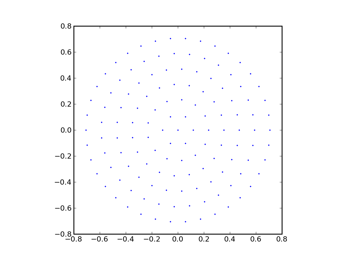
The bundle.py program generates a ray bundle whose appearance is similar to the picture below. This case has 133 rays, attempting to fill out a uniformly-sampled area

The one_3d.py program prints out the intersection points and slopes for every surface, as well as the z-intercept and screen-intercept of the final ray—just like the 2D programs.

Example Output

Using the Petzval lens as an example, we get the following output from one_3d.py:

We used a ray parallel to the optical axis and 5 units away (3-4-5 triangle), and set a screen at the approximate focus of 160 units in z. Because we are operating in 3D, we must report plane intersections rather than axis intersections.

Note the similarity of this result to the 2D analog, where many numbers are identical:

Now we trace this same lens using the bundle.py program. Since so many rays are traced, it no longer makes sense to print out the ray specifics (which is why one_3d.py may still be useful as a diagnostic tool). Instead, here's what we get:

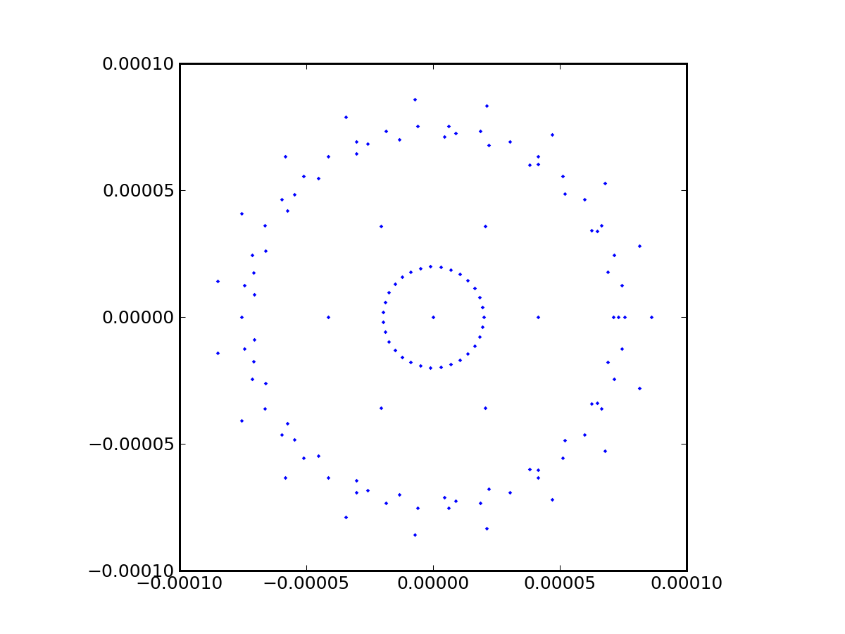
If not specified, the screen finds the best focus (smallest RMS), which is a handy feature so we don't have to hunt around. If you do specify a screen position, the RMS, skew, etc. will be evaluated there. In this case, the best focus has a tiny RMS, but we have yet to put this in context.

We also get a spot diagram in the bargain to show us how the image looks:

Now let's fling rays at it at an angle and get info that we could not possibly get from the 2D case:

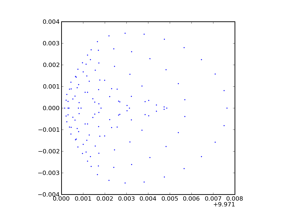
Now we learn some interesting contextual information. If the input ray had a tangent of 0.1 (about 0.1 radians), and the best-focus position was about 10 units up, the effective focal length is about 100 units. The RMS blur is then an angle of 0.0018/100, or about 4 arcseconds, for a fractional blur of 0.018%. In a 16 Megapixel camera (about 4k by 4k, where you are at most 2800 pixels away from center along the diagonal), this corresponds to 0.5 pixels—so the image is still reasonably sharp.

The skew in x indicates an asymmetry, which we see as a strong coma-like appearance in the spot diagram. We also see from this that the maximum extent of the blur is larger than the RMS by a significant factor, so that this effect would begin to show up in the 4k by 4k camera in the previous example, if we wanted it to go all the way to a field angle of 0.1 radians from center.

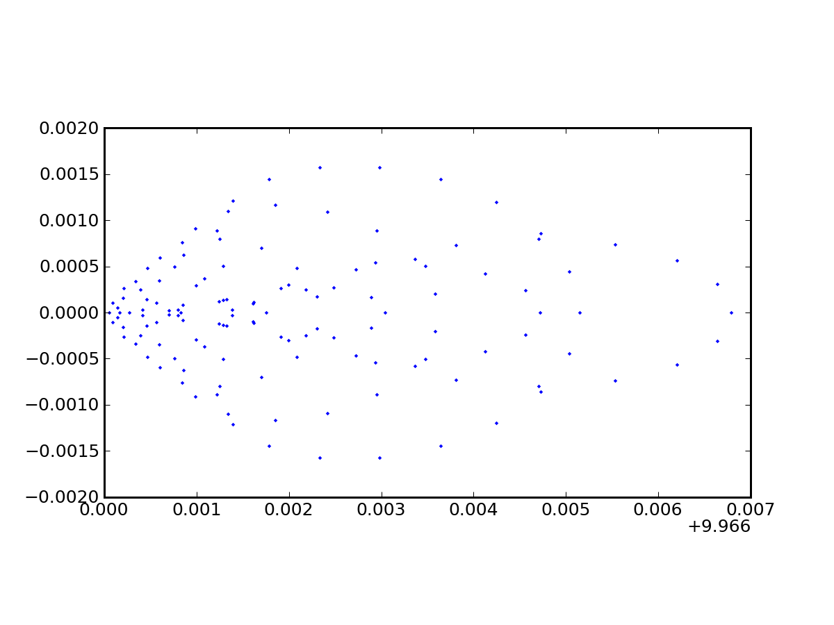
One final exploration: since the image plane is typically flat, how bad is the defocus at a 0.1 degree field angle if the detector is positioned for best focus in the center of the field? For this, we set the screen at 159.115685:

This, predictably, made things a little worse, so that our RMS becomes 5 arcseconds. But the spot diagram is more symmetric (though still skewed seriously, in that most light is on the left), and not horrendously bigger in total scale: 0.008 diameter corresponds to 16 arcseconds for a 100-unit focal length, and would be about 2 pixels across at the edge of a large-format detector.

Example Activities

Many of the examples on the 2D raytrace page can be more richly explored via the 3D package. Assessing aberrations is far easier, and the automatic best-focus feature is convenient as well for exploring field curvature, distortion, etc.

Reflective Systems

The raytracing algorithms (either 2D or 3D, actually), can handle reflective systems. The trick is that the refractive index flips sign on reflection. Initially, we tend to have n = 1.0, which we interpret as: light travels to the right at the speed of light. If we throw in a reflection, we can represent that as saying the new refractive index becomes −1.0, which we interpret as light traveling to the left (negative z, in this context). If we entered glass after the reflection, the index should be something like −1.5, but another reflection would be represented by reversion to +1.0.

For example, a Cassegrain telescope with a 1 meter diameter f2.5 mirror, producing an f/10 focus 0.5 meters behind the primary mirror will need a secondary whose radius of curvature is 1.6 meters. Representing units in millimeters, our prescription becomes:

This prescription eliminates spherical aberration on axis, using a parabolic primary. Evaluating its performance, let's say we want to image the moon onto a 4k×4k CCD with 20 μm pixels. Given the 10 m focal length, the plate scale is 48.5 μm per arcsecond. So the limb of the moon—at 900 arcsec from center, typically—is about 44 mm, or 2200 pixels from field center (will get some chopping at edges unless moon is farther than average). The RMS blur from coma at this angular offset is 28 μm, or 0.6 arcsec. But the full extent of the coma is 0.1 mm, or about 2 arcseconds. By adjusting the conic constant of the secondary mirror to −2.815, we can reduce the coma somewhat, putting most of the light in a 60 μm clump (1.2 arcseconds), while trivially sacrificing spherical aberration at field center (7 μm RMS). But unless we are willing to hyperbolize the primary, as in a Ritchey-Chretien design, we will be stuck with comatic aberration at larger angles.

Topics for Exploration

A collection of topics to explore is available for you to gain experience in investigating optical systems using 3D raytracing.